A few months ago I took a course at my university in computer graphics, which culminated in writing a simple renderer in Python. I’ve rewritten my renderer in C++ as well as adding proper raytraced lighting, and I’ve shared my results (as well as how I reached them) below!

You can check out the source code here.

Some useful resources on raytracing:

• Scratchapixel: Global Illumination and Path Tracing
• Stanford: Monte Carlo Path Tracing
• Wikipedia: Ray tracing
• Wikipedia: Path tracing

A brief introduction to 3D geometry

To understand raytracing we need to familiarise ourselves with a few key ideas in 3D geometry. You can skip this section if you already understand vectors. The code implementing this is in vec3.cpp in the source code.

Vectors

A vector is a quantity with both magnitude and direction. We’re building a 3D renderer so we will be working in the \(\mathbb{R}^3\) vector space - essentially, each vector has 3 real values: \(x\), \(y\), and \(z\).

For the sake of consistency we will define \(x\) to be the horizontal axis, \(y\) to be the vertical axis, and \(z\) to be depth.

From here onwards, all vectors will be written in bold. For example: \(\mathbf{v} = \begin{pmatrix}1 \\ 2 \\ 3\end{pmatrix}\).

When we add together vectors or multiply them by a scalar (regular number), we do so element-by-element:

Magnitude

We can find the magnitude (length) of a vector by using Pythagoras’ theorem:

Normalisation

It often makes it easier to work with vectors if they have a length of \(1\). We can scale a vector to have a length of \(1\) (i.e. normalise the vector) by dividing by its length:

Dot product

The dot product is one method of multiplying vectors, producing a scalar result. The process is very simple - we just multiply element-by-element and add them all together:

The dot product is useful for finding the angle between two vectors, since for any two vectors \(\mathbf{v_1}\) and \(\mathbf{v_2}\) the following rule holds (where \(\theta\) is the angle between the vectors):

This has the nice side-effect that the dot product is \(0\) when the two vectors are perpendicular.

Cross product

The cross product is another method of multiplying vectors, this time producing a vector result. The resulting vector is perpendicular to both the original vectors, and obeys the following rule (where \(\theta\) is the angle between the two vectors, and \(\mathbf{n}\) is the normalised vector perpendicular to the original two):

Computing the cross product is a bit more complicated. Here’s the formula for doing so:

Primitives

Now we have a basic idea of 3D geometry we need to define primitives for any shape we want to render. In this example program we’re implementing sphere and triangle primitives. For each of these we need to implement intersect and normal functions. The first returns the intersection of a ray with the shape (if such an intersection exists) and the second returns the normal of the primitive at a given point. Both primitives will inherit from the following abstract class:

class Primitive {
public:
    virtual float intersect(vec3 origin, vec3 direction) = 0; // Returns t1 such that the ray intersects at origin + (t1 * direction)
    virtual vec3 normal(vec3 location) = 0; // Returns the normal at location, negative if no intersection
};

Sphere

We will define a sphere in terms of its origin \(\mathbf{c}\) and radius \(r\), with a constructor that takes both these values:

Sphere::Sphere(const vec3 origin, float radius) {
    origin_ = origin;
    radius_ = radius;
}

Intersection

Ray-sphere intersection is somewhat complicated, but the code is relatively straightforward. Scratchapixel has a great explanation of the mathematics here. The code that implements this test is as follows (note that we use a negative value to mean no intersection):

float Sphere::intersect(vec3 origin, vec3 direction) {
    vec3 L = origin_ - origin;
    float tc = L.dot(direction);

    if (tc < 0) {
        return -1.0;
    }

    float d2 = L.magnitude_squared() - (tc * tc);
    float radius2 = radius_ * radius_;

    if (d2 > radius2) {
        return -1.0;
    }

    float t1c = sqrt(radius2 - d2);
    float t1 = tc - t1c;
    // t2 = tc + t1c;

    return t1;
}

Normal

The normal of a sphere is very straightforward - assuming a point \(\mathbf{p}\) is on the surface of the sphere, the normal at \(\mathbf{p}\) is the normalised distance between it and the centre of the sphere: \(\frac{\mathbf{p}-\mathbf{c}}{\lVert \mathbf{p}-\mathbf{c} \rVert}\).

vec3 Sphere::normal(vec3 location) {
    return (location - origin_).norm();
}

Triangle

Triangles are defined in terms of each of their vertices: \(\mathbf{v_0}\), \(\mathbf{v_1}\), and \(\mathbf{v_2}\). Since triangles are flat we can also compute the normal at this step by taking the cross product of two of its edges.

Triangle::Triangle(const vec3 p0, const vec3 p1, const vec3 p2) {
    p0_ = p0;
    p1_ = p1;
    p2_ = p2;
    normal_ = (p1_ - p0_).cross(p2_ - p0_).norm();
}

Intersection

Computing the intersection of a ray with a triangle is a bit more complicated than with a sphere. We first compute the intersection with the plane in which the triangle lies, then figure out if that point lies within the triangle or not. Once again, Scratchapixel has an in-depth explanation here and the relevant code is below:

float Triangle::intersect(vec3 origin, vec3 direction) {
    vec3 edge1 = p1_ - p0_;
    vec3 edge2 = p2_ - p0_;

    vec3 h = direction.cross(edge2);
    float a = edge1.dot(h);
    if (a > -EPSILON && a < EPSILON)
        return -1;

    float f = 1.0/a;

    vec3 s = origin - p0_;
    float u = f * s.dot(h);
    if (u < 0.0 or u > 1.0)
        return -1;

    vec3 q = s.cross(edge1);
    float v = f * direction.dot(q);
    if (v < 0.0 or u + v > 1.0)
        return -1;

    float t = f * edge2.dot(q);
    if (t > EPSILON && t < 1/EPSILON)
        return t;

    return -1;
}

Normal

Since we already computed the normal, we just return that value - we assume any calls to normal pass in a point within the triangle.

vec3 Triangle::normal(vec3 location) {
    return normal_;
}

The basic renderer

Now that vectors and primitives have been implemented, we can write a basic renderer. This renderer will cast out rays corresponding to each pixel of the output image and check for intersections with each object in the scene. We do not have any lighting yet, so we will colour pixels black and white.

Raycasting

First we need to write a raycast function which, given an origin and direction, checks intersection with all objects in the scene. This is fairly easy to implement, but it requires us to add a new Intersection class since we need the object as well as the intersection point. We can see this and the main raycast code below:

class Intersection {
public:
    Primitive *object;
    float t;
    vec3 point;
    bool success;
};

Intersection Renderer::raycast(vec3 origin, vec3 direction) {
    Intersection result;
    result.t = FLT_MAX;
    result.success = false;
    for (auto const& prim : scene_) {
        float t = prim->intersect(origin, direction);
        if (t > 0.0 && t < result.t) {
            result.object = prim;
            result.t = t;
            result.point = origin + direction*t;
            result.success = true;
        }
    }
    return result;
}

The Camera

In the constructor for the renderer we defined the camera’s location, direction, up vector, and field of view. Now we need to use this to generate a grid of rays originating from the camera. We’ll space out the rays evenly by adding a fixed amount of the camera’s left and up vector each time. To figure out how much to add at the most extreme points we solve the following triangle:

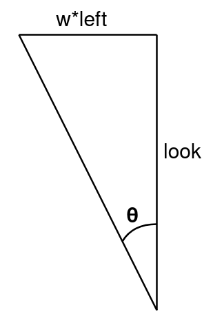
Since we know look and left have magnitude 1 (and are perpendicular) and \(\theta\) is fov/2, we get w = tan(fov/2). We use the same value for the vertical offset as well, correcting for the image’s ratio:

left_ = up.cross(look).norm();
w_ = h_ = tan(fov/2);
float ratio = (float)height_ / (float)width_;
if (ratio < 1.0) {
    h_ *= ratio;
}
else {
    w_ /= ratio;
}

Image Generation

Now we have a camera, objects in the scene, and a raycast function - all that remains is to turn it into an image! For this we’ll be using the CImg library, which allows us to write an image pixel-by-pixel and output the result to a file. For each pixel we use the camera parameters derived above to generate a direction vector, and use raycast to figure out if there has been an intersection. We’ll also write get_colour and set_colour helper functions to make it easier to extend once we add lighting:

Colour Renderer::get_colour(Intersection &in) {
    if (in.success) {
        return Colour(0,0,0);
    }
    else {
        return Colour(255,255,255);
    }
}

void Renderer::set_colour(CImg<unsigned char> &img, int x, int y, Colour colour) {
    img(x,y,0) = colour.r;
    img(x,y,1) = colour.g;
    img(x,y,2) = colour.b;
}

void Renderer::render() {
    CImg<unsigned char> output(width_, height_, 1, 3);
    for (int i = 0; i < width_; i++) {
        for (int j = 0; j < height_; j++) {
            float a = w_ * (((float)i - ((float)width_ / 2)) / ((float)width_ / 2));
            float b = (-1.) * h_ * (((float)j - ((float)height_ / 2)) / ((float)height_ / 2));
            vec3 dir = (look_ + left_*a + up_*b).norm();
            Intersection in = raycast(camera_, dir);
            set_colour(output, i, j, get_colour(in));
        }
    }
    output.save("render.png");
}

First Render

Now all we need to do is set up a basic scene with some shapes to get a render:

int main() {
    int width = 1920;
    int height = 1080;
    vec3 camera = vec3(0,0,0);
    vec3 look = vec3(0,0,1);
    vec3 up = vec3(0,1,0);
    float fov = 1.22; // approximately 70 degrees
    Renderer renderer = Renderer(width, height, camera, look, up, fov);

    Sphere s = Sphere(vec3(0.5, 0.5, 7), 1.2);
    renderer.add_primitive(&s);
    Triangle t = Triangle(vec3(-3, 1, 7), vec3(-1, 1, 7), vec3(-3, 4, 9));
    renderer.add_primitive(&t);

    renderer.render();

    return 0;
}

This gives us the following image:

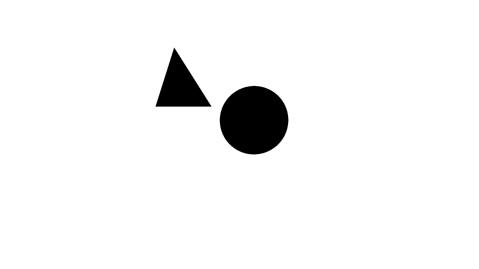Success!

Lighting

The renderer works just fine so far, but everything is flat! To fix this we need to add some lights to the scene and start doing some basic lighting calculations.

We’ll start by adding an abstract Light class, plus AmbientLight and PhongLight classes which implement this - much like our Primitives earlier on. Each light has an illumination function which takes an Intersection and returns the colour at that intersection as a vector. We’re using vec3 to store and process colours, and only transforming into an unsigned char (range 0-255) right at the end - this allows us to have more precision when working.

Ambient lights are the most straightforward - the constructor takes a colour, and the illumination by that light at any point is always that colour. These lights are used to approximate light reflected off other objects in the scene, and we’ll remove them once we implement proper raytraced lighting.

AmbientLight::AmbientLight(const vec3 colour) {
    colour_ = colour;
}

vec3 AmbientLight::illumination(Intersection &in) {
    return colour_;
}

For our Phong lights we need to introduce some new coefficients on our primitives - we’ll be using the following equation to calculate illumination:

\(I_p\) is the light’s colour, \(k_*\) are coefficients specific to the object being lit, \(\mathbf{N}\) is the surface normal, \(\mathbf{L}\) points from the surface to the light, \(\mathbf{R}\) points in the direction of light reflected off the surface, and \(\mathbf{V}\) points towards the viewer (or the ray’s origin in the case of reflected rays). Note that all vectors must be normalised. By tweaking these coefficients we can get a decent approximation of many different materials.

Here’s the code that implements this lighting calculation:

vec3 PhongLight::illumination(Intersection &in, vec3 &origin) {
    vec3 colour = vec3(0.,0.,0.);
    vec3 N = in.object->normal(in.point);
    vec3 L = (pos_ - in.point).norm();
    vec3 R = N * (2 * N.dot(L)) - L;
    vec3 V = (origin - in.point).norm();
    float diffuse = N.dot(L);
    float specular = R.dot(V);

    if (diffuse < 0)
        diffuse = 0;
    if (specular < 0)
        specular = 0;

    colour = colour_ * (in.object->phong_diffuse * diffuse + in.object->phong_specular * pow(specular, in.object->phong_exponent));

    return colour;
}

Now all we have to do is modify the renderer’s get_colour function to get the illumination from each light:

vec3 Renderer::get_colour(Intersection &in) {
    if (in.success) {
        vec3 colour = vec3(0., 0., 0.);
        for (auto const& light : lights_) {
            colour += light->illumination(in, camera_);
        }
        return colour;
    }
    else {
        return vec3(1., 1., 1.);
    }
}

Once we add some lights to our scene this can give us some much nicer renders!

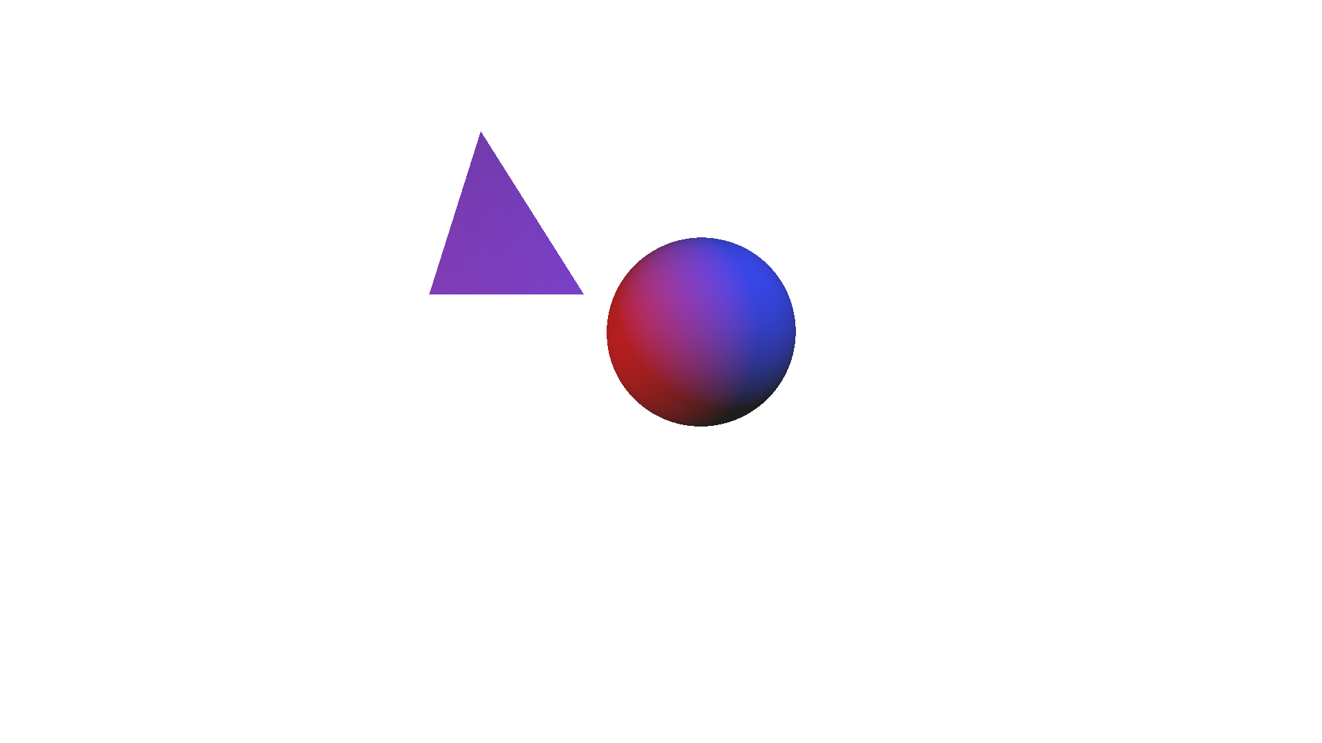Check it out!

By modifying the diffuse and specular components of a material we can change how it looks:

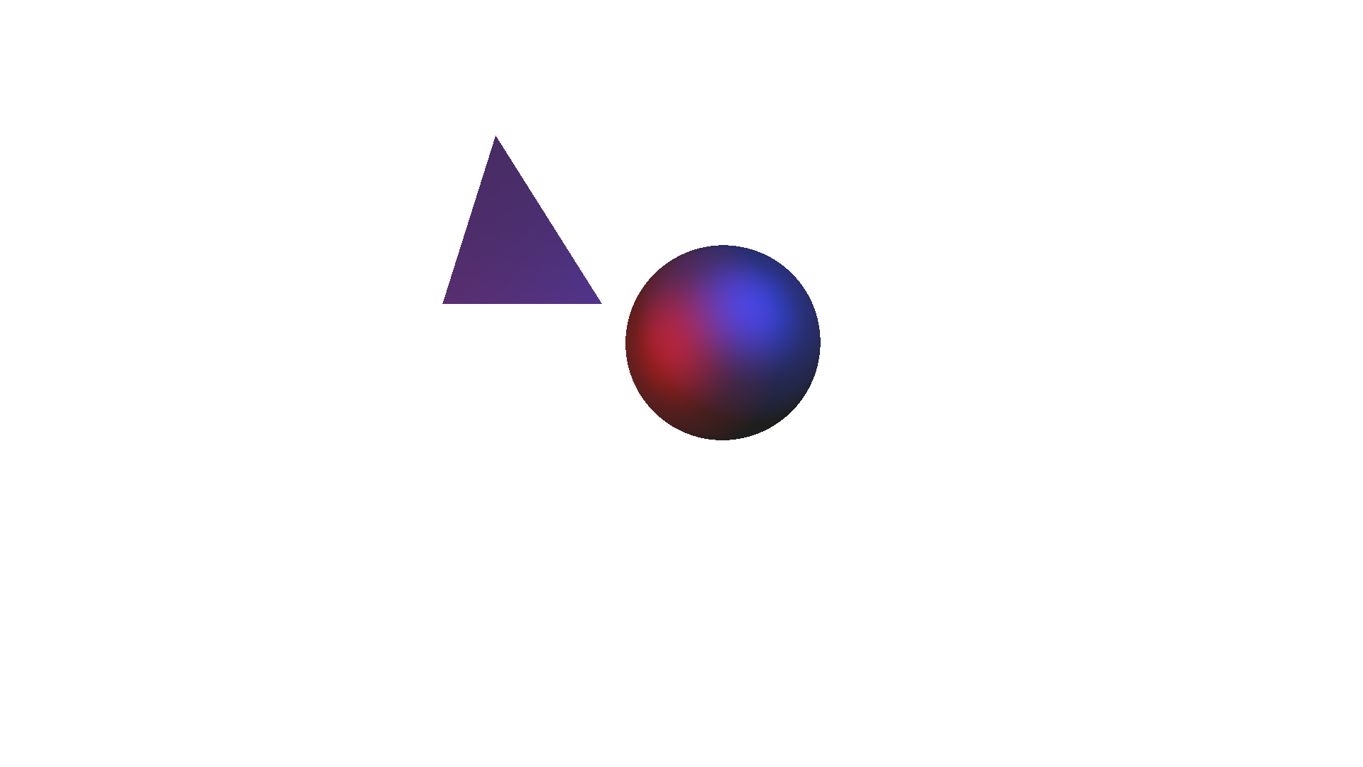Oooh, metallic!

Path Tracing

While we can get some solid renders out of what we’ve got so far, it’d be a shame to build a raytracing renderer without using its raytracing ability to do some more advanced processing - what we’ve got so far is hardly better than a standard rasterising renderer. We can get far better (although more expensive) lighting calculations by sending off more rays each time a ray collides with an object to compute the final colour of a pixel.

We don’t just want to fire off rays completely at random - that would make every pixel a grainy mess! Instead we want to randomly sample the reflectance model used above to generate outgoing rays, so the resulting colour approximates the result of the reflectance model.

First we write helper functions to randomly sample the diffuse and specular portions of the Phong reflectance model - this article explains how the maths behind this works. From this we get the following code:

vec3 sample_diffuse(vec3 normal) {
    float theta = acos(sqrt(random01()));
    float phi = 2 * M_PI * random01();
    return spherical_to_vector(normal, theta, phi);
}

vec3 sample_specular(vec3 reflected, float exponent) {
    float alpha = acos(pow(random01(), 1/(exponent+1)))
    float phi = 2 * M_PI * random01();
    return spherical_to_vector(reflected, alpha, phi);
}

This code was later revised to aid with lighting calculations, instead returning the computed angles with the vector computed by the renderer.

spherical_to_vector converts spherical coordinates to a vector relative to a given normal, and random01 generates a random float between 0 and 1.

When path tracing we incorporate the lighting calculations into the main process, so we no longer use the get_colour function. Instead we call a new pathtrace function which recursively traces the path of a ray to compute a pixel’s colour. Since this process has a high degree of randomness the resulting image is very grainy - to mitigate this, we trace many paths and average the result. This gives us the following render code for each ray:

vec3 colour = vec3(0., 0., 0.);
for (int i = 0; i < samples; i++) {
    colour += pathtrace(camera_, dir, 0, maxdepth);
}
colour /= samples;
set_colour(output, i, j, colour);

Our pathtrace function traces the path of a single ray through the scene, returning black if the maximum depth is exceeded and computing lighting if the ray exits the scene. The code is as follows:

vec3 Renderer::pathtrace(vec3 origin, vec3 direction, int depth, int maxdepth) {
    if (depth >= maxdepth) {
        return vec3(0,0,0); // the ray has bounced too many times, return black
    }

    Intersection in = raycast(origin, direction);
    if (!in.success) { // ray has left the scene
        if (depth == 0) {
            return background_; // if this is the very first bounce, return the background colour
        }
        else {
            // the ray has already bounced off at least one object, do basic directional lighting calculations
            vec3 colour = vec3(0., 0., 0.);
            for (auto const& light : directional_lights_) {
                colour += light->colour * clamp(direction.dot(light->dir * (-1)));
            }
            return colour;
        }
    }

    // Pick a new ray (assuming phong_diffuse + phong_specular = 1)
    float r = random01();
    vec3 normal = in.object->normal(in.point);
    vec3 direction2;
    if (r < in.object->phong_diffuse) { // selected ray contributes to diffuse reflection
        float theta = sample_diffuse1();
        float phi = sample_diffuse2();
        direction2 = spherical_to_vector(normal, theta, phi);
    }
    else { // selected ray contributes to specular reflection
        vec3 reflected = normal * (2 * normal.dot(direction.norm())) - direction.norm();
        float alpha = sample_specular1(in.object->phong_exponent);
        float phi = sample_specular2();
        direction2 = spherical_to_vector(reflected, alpha, phi);
    }
    vec3 R = normal * (2 * normal.dot(direction2)) - direction2;
    float contribution = in.object->phong_diffuse * clamp(normal.dot(direction2)) + in.object->phong_specular * clamp(R.dot(direction));

    vec3 incoming_colour = pathtrace(in.point, direction2, depth+1, maxdepth);

    return incoming_colour * in.object->colour * contribution;
}

This may look a little complicated, but most of the code is simply calculating the new ray’s parameters. When pathtrace returns the colour from the new ray, we treat it as a light source and use it to compute the pixel’s resulting colour (this is what contribution is for).

Rendering

Now we have our new render function, all we need to do is set up a new scene with some objects and at least one directional light source! In this example render I’ve added some spheres of different colours to demonstrate the new lighting:

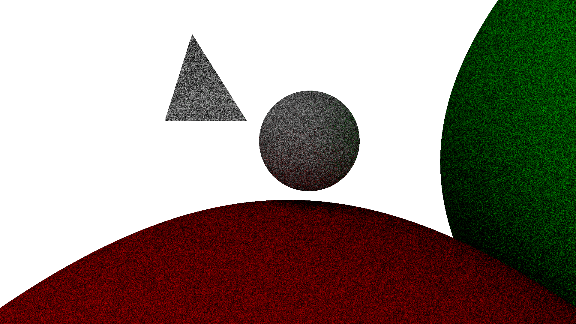Grainy but fast

As mentioned earlier, we can increase the quality of the render by taking more samples per pixel. These renders will take a lot longer, but they look a lot smoother!

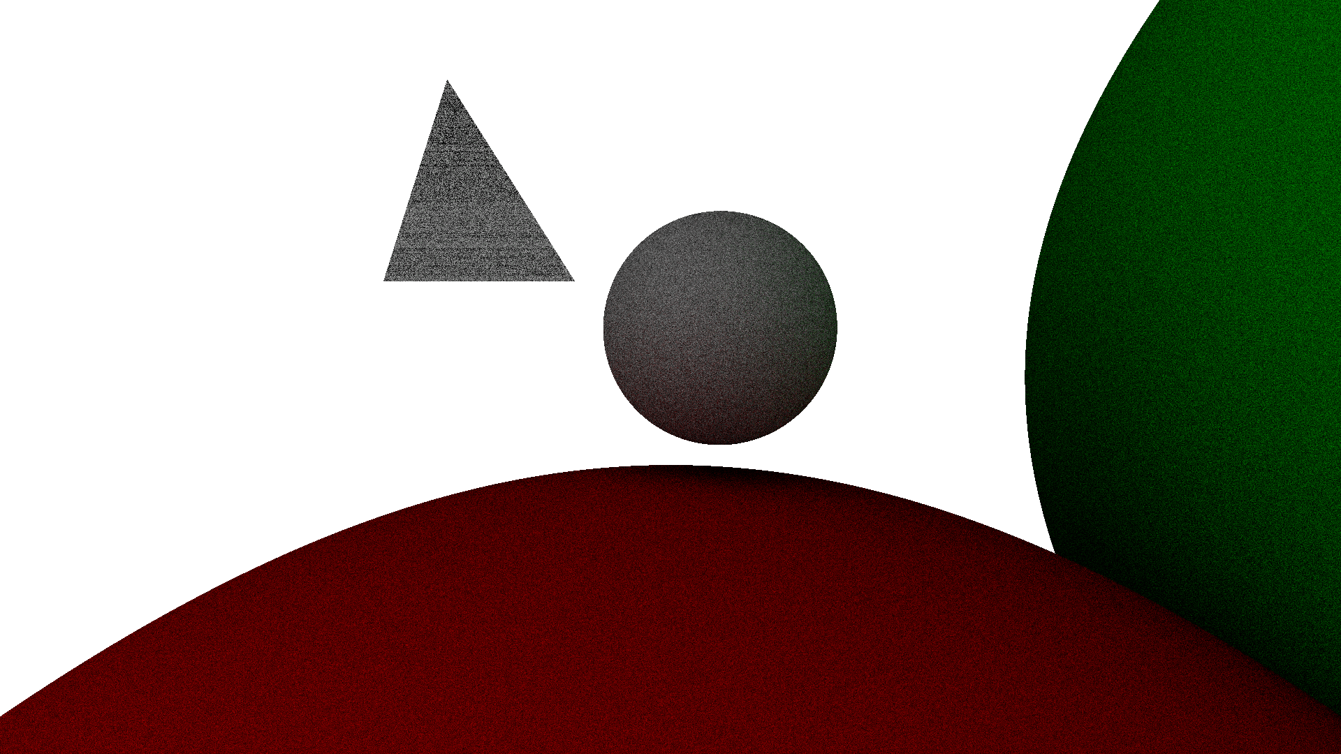Less grainy (8 samples per pixel)

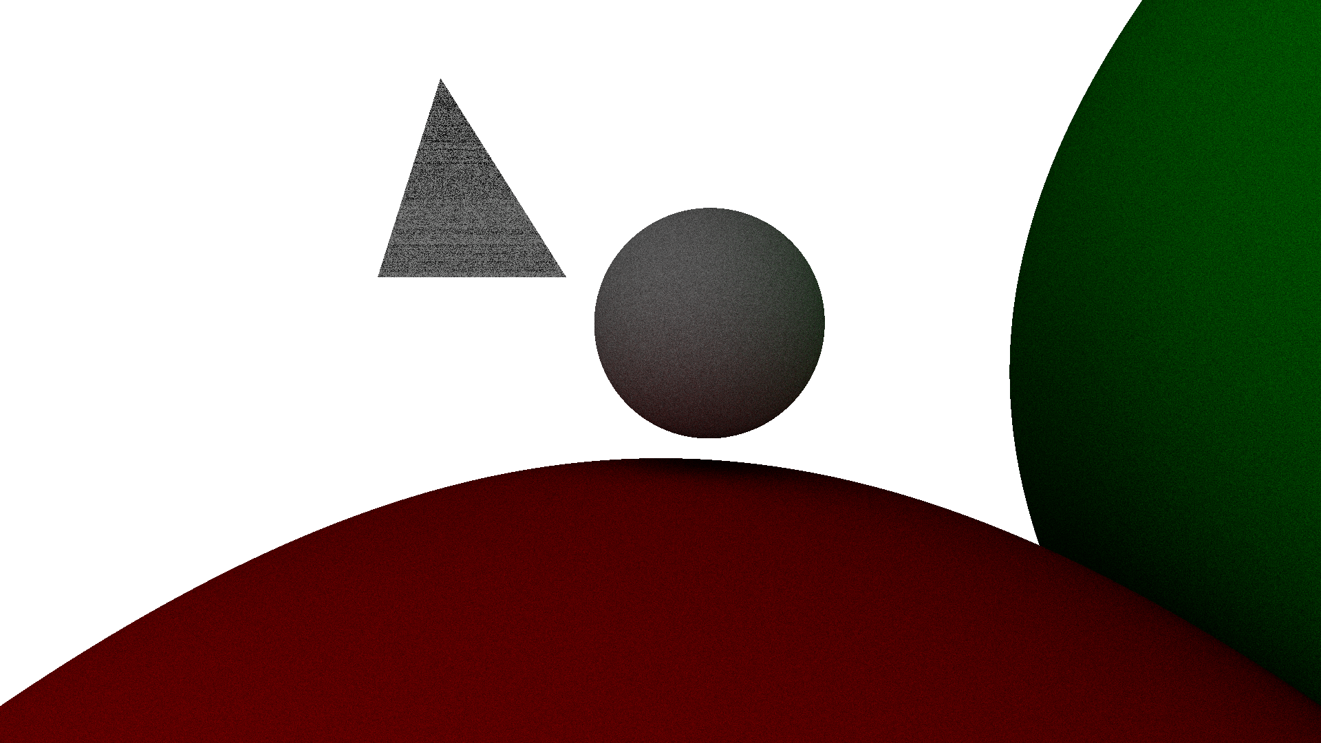Even smoother (32 samples per pixel)

We can look at the smaller sphere to see that the lighting is working correctly - the red sphere is casting a subtle red glow on the lower portion of the sphere, and the same is happening on the right edge with the green sphere!

Conclusion

Implementing this basic renderer taught me a lot about how this style of rendering works, as well as helping me to get slightly better at working with C++. While the renderer is far from fast (single thread CPU-bound, not written with efficiency in mind) I hope it can be a somewhat useful reference material. Far better raytracing renderers already exist (check out the Blender project’s Cycles renderer), but their feature set is so large that it would be quite a task for a beginner to understand the source code. I hope this is a useful middle ground!

There are a number of features that could be implemented to extend this renderer, and I may add some of them in the future:

• Importing meshes from .obj files so actual scenes can be rendered
• Mirrored surfaces (should be fairly straightforward, simply reflect the ray without scattering when path tracing)
• Transparent or translucent surfaces, simulating refraction and internal reflection

In the meantime, check out the source code here. I hope you learned something from this post!